IFM — Imaging/Display (for LBS)
A short history of LBS
Laser Beam Scanning (LBS) display systems emerged to shrink optics and drive pixels by steering a narrow beam rather than addressing a 2-D array. Early LBS used galvanometers or polygon scanners; MEMS mirrors later enabled smaller, faster, lower-cost engines that fit wearables, pico-projectors, HUDs, and lighting.
Where conventional MEMS-based LBS struggles
Limited optical throughput.
Tiny mirrors often force single-mode lasers and limit brightness.
Thermal constraints.
Monolithic mirrors run hot at higher optical power.
Shock/vibration vs. size.
Large single mirrors become fragile; reliability suffers.
Integration overhead.
Drive electronics and feedback add cost and size.
video from internet
Despite this, LBS is still the most economical path to a projection display because it avoids costly 2-D emitters/modulators and large projection optics.
inSync’s approach
IFM use synchronized mirror units. Each unit has its own hinges, anchors, actuators, and mirror. Many units move in lockstep at resonance, so they behave like one large effective aperture.
What this means from the MEMS side
Aperture scaling without extra inertia.
Unit size stays constant, so rotational momentum per unit doesn’t balloon while total aperture scales.
Efficient heat dissipation.
Every unit conducts heat through its own hinge/anchor into the substrate, improving thermal handling.
High mechanical bandwidth.
Fast-axis resonant operation around ~20 kHz supports stable scanning at display refresh rates.
Standardizable building blocks.
Keep the unit process stable and scale effective area by synchronization, not by risky monolithic upsizing.
What this means for an LBS projector
Higher brightness and support for multi-mode lasers.
Larger effective aperture passes more light and tolerates higher optical power.
Better eye safety at a given lumen level.
Larger spot/area lowers peak irradiance.
High reliability.
Many small moving masses are more shock/vibe-robust than one big mirror.
Lower system cost at scale.
Reuse standard mirror units; scale with synchronization.
Typical IFM configurations
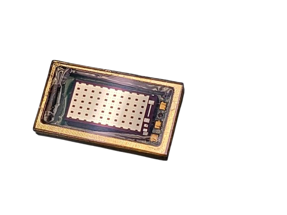
IFM-1D
Fast axis, resonant scanner
Pair with a slow axis to form a 2-D scanner.
6mm × 3mm active optical area, 20kHz.
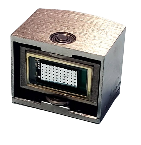
IFM-2D
Hybrid scanner
Resonant fast axis MEMS sitting on electromagnetically driven slow axis.
Up to 40Hz triangle wave scanning.
IFM key parameters (customizable)
Most parameters can be tailored (aperture, scan angle, coatings, sensing, package, drive). Values below reflect current IFM prototypes/typicals.
| Parameter | Condition / Notes | Min | Typ | Max | Unit |
|---|---|---|---|---|---|
| Optical effective aperture (1D mirror) | Illuminated area | — | 15 | — | mm² |
| Optical scan angle (fast axis) | Optical, p-p | — | 30 | — | ° |
| Reflected-beam divergence | Collimated, λ = 635 nm, full aperture | — | 2 | 3 | mrad |
| Resonant frequency (fast axis) | Room temp, 1 atm | 18 | 20 | 22 | kHz |
| Power (fast-axis drive) | At typical optical angle | 0.5 | 0.8 | 1.0 | mW |
| Drive voltage (fast axis) | Sinusoidal, Vpp at typical angle | 80 | 110 | 140 | V |
| Drive current (fast axis) | At typical angle | 200 | 300 | 400 | µA |
| Mechanical Q (fast axis) | 1 atm | 160 | 190 | 210 | — |
| Angle detection noise | RMS optical angle | — | 0.002 | — | ° |
| Angle detection accuracy | −40 ~ 85 °C | — | 0.01 | 0.05 | ° |
| Mirror reflectivity | 450–650 nm | 95 | 97 | — | % |
| G-shock resistance | Half-sine, 0.5 ms, 3-axis, 3× each | 1500 | — | 6000 | g |
| Slow-axis optical angle (2D hybrid) | Quasi-static | — | 50 | — | ° |
| Slow-axis control accuracy | 60 Hz triangular | — | 0.04 | — | ° |
| Slow-axis power | Averaged | — | 0.2 | — | W |
| Slow-axis max voltage / current | Stall at peak | — | 6 / 0.3 | — | V / A |